The volume-FMM workflow#

A volume potential

\[ u(\boldsymbol{x}) = \int_{\Omega} G(\boldsymbol{x}, \boldsymbol{y})\, f(\boldsymbol{y})\,\mathrm{d}\boldsymbol{y} \]

is not a particle sum. Where the target lies inside the source box the integrand is genuinely singular and the tensor-product point quadrature used for the far field does not resolve it; in the neighbouring boxes it is finite but near-singular, and that quadrature converges too slowly to be useful at the orders the method runs at. Volumential’s answer to both is the same: split the domain by distance in the tree rather than by quadrature rule.

Far field — boxes well separated from the target — is an ordinary particle FMM over the volume quadrature nodes, weighted by the quadrature weights. Nothing about it is volume-specific.
Near field — the target’s own box and its List 1 neighbours — is read from a table of precomputed integrals, one entry per (source mode, target node, interaction case): singular ones for the self box, near-singular ones for the neighbours, all built once by desingularizing quadrature.

The code calls this fpnd: far field by particle approximation, near field direct. Every wrangler in volumential.wranglers implements it; the two backends differ only in who produces the far field.

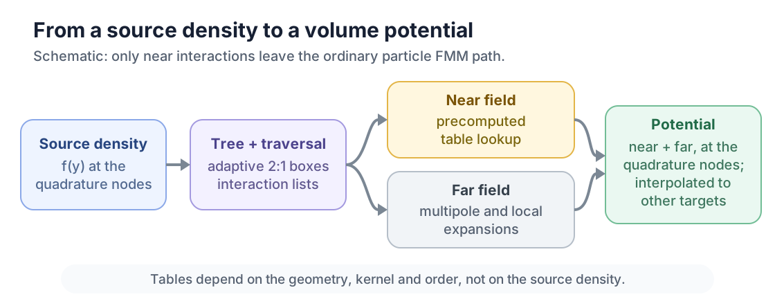
Schematic flow chart. The source density at the box quadrature nodes goes into a tree with its traversal, then splits into a near-field path, a precomputed table lookup, and a far-field path, ordinary FMM expansions; the two paths add up to the potential. — Schematic, not computed output: the whole computation in one picture. The stages below name the objects and modules behind each box.#

Stages#

1. A box mesh and its quadrature nodes#

volumential.meshgen builds a box-shaped mesh over a cube and places tensor-product Gauss-Legendre nodes of order q_order in each leaf. MeshGen1D/2D/3D expose the nodes (get_q_points, shape (nnodes, dim)) and weights (get_q_weights) on host or device.

Adaptive refinement and coarsening of the underlying tree of boxes, including the 2:1 level restriction that keeps List 1 bounded, live in volumential.tree_interactive_build. What that restriction allows in List 4, and what it costs in accuracy, is in On a graded tree. Refinement is driven by a user-supplied per-leaf criterion, so a source that is tight in one corner of the domain does not force a uniform tree everywhere. examples/laplace2d_adaptive.py refines by a resolution criterion on the source and compares the result with a uniform tree with at least as many leaves (laplace2d_adaptive.py).

volumential.geometry assembles the objects the wranglers actually consume: BoundingBoxFactory for the root box, BoxFMMGeometryFactory for the repeated build, and the resulting BoxFMMGeometryData (nodes, weights, tree, traversal).

2. A tree and a traversal#

The nodes are handed to boxtree’s TreeBuilder, normally with kind="adaptive-level-restricted" and max_particles_in_box set from q_order**dim, so that one leaf holds one element’s worth of nodes. FMMTraversalBuilder then produces the interaction lists.

Two details bite:

Pass targets=None when the targets are the source nodes. Building a traversal from separate-but-identical arrays gives a different, subtly wrong self-interaction structure; VOLUMENTIAL_STRICT_SOURCE_TARGET_TREE=1 turns that into an immediate failure (see Device selection).
The boxtree version matters. A stale refine_and_coarsen_tree_of_boxes corrupts List 1 on reordered adaptive trees without any error; the check in Installation is what catches it.

3. A near-field interaction table#

volumential.table_manager.NearFieldInteractionTableManager is the entry point. get_table(dim, kernel_type, q_order, ...) returns a table, building it on a cache miss and loading it from SQLite otherwise.

The table holds, for each List 1 interaction case (the relative position of the source box to the target box, as a case vector) and each pair of source mode and target node, the integral of the kernel against that source basis function. Those integrals are singular on the self box and near-singular on the neighbours, and volumential.nearfield_potential_table evaluates them with Duffy-type radial desingularization quadrature in 2D and 3D; volumential.singular_integral_2d carries an older 2D-only Duffy implementation specialized to 1/r-type kernels.

A table is keyed by the kernel, the dimension, q_order and the source_box_level — that is what TableRequest carries — plus the build configuration, which the cache fingerprint hashes. It does not depend on the source density, on the tree’s topology, or on the target points.

The root_extent is not part of that key. It is a property of the cache file as a whole: the manager stores it in the database on first write and raises if a later manager opens the same file with a different value. That is the right behaviour, because the integral values — and the Helmholtz/Yukawa parameter scaling on top of them — are tied to the box extent. The practical consequence is that a second root extent needs a separate cache file, not a second key in the same one.

Building the table is by far the largest one-time cost, which is why the cache file is worth keeping. How a build is routed, and how to tell after the fact which path produced a cached table, is Near-field table build routing.

The table is stored symmetry-reduced. volumential.list1_symmetry discovers the symmetry operations the kernel and dimension admit, volumential.orbit_arithmetic canonicalizes entries under them, and only canonical entries are stored; volumential.list1_gallery enumerates the cases. See Near-Field Symmetry Reduction for the storage format and the runtime reconstruction, and ORBIT canonicalization for why the arithmetic variant exists.

Fixed-parameter Helmholtz and Yukawa tables can also be assembled from a parameter-independent channel family instead of being built by quadrature per parameter; that is volumential.rke_table_assembly and Windowed singular channels and certified assembly.

4. A wrangler#

volumential.expansion_wrangler_interface states the interface the driver calls. volumential.wranglers implements it twice:

FPNDExpansionWrangler / FPNDSumpyExpansionWrangler — expansions generated by sumpy. Works for every kernel sumpy can differentiate, and carries the near-field Helmholtz split.
FPNDFMMLibExpansionWrangler — expansions from pyfmmlib through boxtree.pyfmmlib_integration. Restricted to 2D/3D Laplace and Helmholtz, to a tree whose sources and targets coincide, and considerably faster given the environment of Installation. Two separate properties of that build matter, and confusing them misdiagnoses a slow run: without OpenMP the rotation M2L runs on one thread, and — for charge sources — without the batched {l,h}{2,3}dformmp_imany wrappers form_multipoles silently drops to a serial per-box P2M. (A DirectionalSourceDerivative configuration sets use_dipoles, which bypasses that lookup entirely and takes boxtree’s inherited dipole path, so those four symbols say nothing about it.) Neither announces itself.

Which one to prefer is not obvious and depends on the device as much as on the kernel — on a CPU OpenCL device a 3D Helmholtz solve at high order is 99 % sumpy’s FFT-based M2L, and FMMLib with an OpenMP pyfmmlib is about 9x faster on the same hardware, while a current GPU runs the sumpy path in seconds. Choosing a wrangler has the measurements and the caveats.

Both share the near-field machinery: table marshalling (volumential.wranglers.table_data), orbit reconstruction (volumential.wranglers.arithmetic_orbits, volumential.wranglers.orbit_generated), and the on-device List 1 evaluators in volumential.list1 (NearFieldFromCSR reads table data through the CSR interaction lists the traversal produced).

volumential.expansion_wrangler_fpnd is a compatibility shim: every name that was importable from it before the split is re-exported and refers to the same object, so the historical import path keeps working. It is not a mirror of the current package — names added since, the mixins FMMLibBatchedStagesMixin, HelmholtzSplitCorrectionMixin and NearFieldPayloadCacheMixin among them, exist only in volumential.wranglers. New code should import from there.

5. Drive it#

volumential.volume_fmm.drive_volume_fmm() runs the two FMM passes and adds the near-field stage:

(pot,) = drive_volume_fmm(trav, wrangler, src_weights, src_func)

src_weights is the source density times the quadrature weights (what the far field integrates); src_func is the bare density (what the near-field table contracts against). Passing the same array for both is a common and quiet error.

direct_evaluation=True replaces the whole evaluation with a global point-to-point sum over the quadrature nodes (sumpy’s P2P), and returns before the List 1 stage runs — it does not use the near-field tables. Two limits, and neither is checked for you. It is sumpy-only: the branch reaches wrangler.tree_indep._setup_actx, which only the sumpy backend sets, so an FMMLib wrangler raises AttributeError there after having already formed multipoles. And it wants a coincident source/target tree: the branch passes target_to_source = arange(tree.ntargets) unconditionally, so with distinct target arrays and exclude_self=True target i drops source i even though the two are unrelated points, and it bypasses the automatic interpolation below as well. It is a diagnostic for the far-field path, not an accuracy oracle for the near field: point quadrature does not resolve the singular near-field integrand, so a disagreement with it says nothing on its own. The reference the near-field accuracy checks actually use is a table comparison — direct per-level tables against a rescaled canonical level-0 table, and both against a manufactured solution.

timing_data={} collects the per-stage times drive_volume_fmm records through its TimingRecorder. The per-phase shares are a separate API: build a volumential.phase_profile.PhaseProfile, activate it around the solve with volumential.phase_profile.profiling(), and call its shares() method. That path synchronizes the OpenCL queue at phase boundaries, so its numbers have different semantics from the timing_data stage times and the two are not interchangeable.

6. Get the values where you want them#

What drive_volume_fmm returns depends on the tree it was given. With a coincident source/target tree — the usual case, and the one the example builds with targets=None — it returns the potential at the box-mesh nodes. When the traversal carries distinct target arrays and the wrangler is a sumpy one, the default auto_interpolate_targets=True does the second step for you: it solves on the source modes, interpolates to tree.targets, and returns values in the requested target layout. Interpolating that result again is a shape error waiting to happen. The branch is guarded by isinstance(expansion_wrangler, FPNDSumpyExpansionWrangler), so an FMMLib wrangler does not take it — and does not reach an output layout either: it continues through the traversal as given and _compute_box_local_ids raises ValueError in the List 1 stage, because table-based near-field evaluation requires tree.sources_are_targets. The automatic path is therefore sumpy-only; FMMLib reaches distinct targets only through the manual route of Choosing a wrangler — a source-only coincident solve followed by volumential.volume_fmm.interpolate_volume_potential().

volumential.volume_fmm.interpolate_volume_potential() evaluates a box-mesh potential at an arbitrary set of target points — the explicit form of what the automatic path does.
volumential.interpolation transfers between the box mesh and a meshmode discretization in both directions, which is how Volumential couples to a pytential boundary-integral solve (see examples/poisson3d.py).

The interpolation is \(O(N \log N)\), but in practice indistinguishable from \(O(N)\): the geometry lookup is a very small fraction of the runtime.

Sources#

The density does not have to arrive as an array.

volumential.symbolic and volumential.tools.ScalarFieldExpressionEvaluation evaluate a pymbolic expression at the quadrature nodes on device. This is what the examples use.
volumential.gaussian supplies Gaussian fixtures with closed-form potentials, which is what most accuracy checks measure against.
volumential.function_extension continues a density given on a curved domain to the surrounding box using layer potentials, so that the extended values can be evaluated directly at volume quadrature targets. That is the route from a Poisson problem on a non-box domain to a volume potential on a box.

Kernels#

Laplace, Helmholtz and Yukawa are supported in 2D and 3D for potential and target gradient; see M1 Kernel Coverage for the matrix and Derivative Support for the derivative wrappers and their sign bookkeeping.

Helmholtz and Yukawa additionally support the near-field split, which subtracts the smooth part of the kernel so that one Laplace-like table family serves a whole range of parameters instead of one table per wave number. That is Helmholtz Split Formulation.

Where the time goes#

Roughly, in a first run: table build, then sumpy code generation for the first solve, then the FMM itself. In a warm run the table is a millisecond-scale load and the code-generation cache is hit, so the FMM dominates. Any timing claim therefore has to separate first-call from warm seconds and say which device class it ran on — Benchmarks and reproducibility is the rest of what it has to record.