Volumential#
Volumential evaluates volume potentials, integrals of a kernel against a source density over a box, with the Fast Multipole Method. This is what the first example computes.
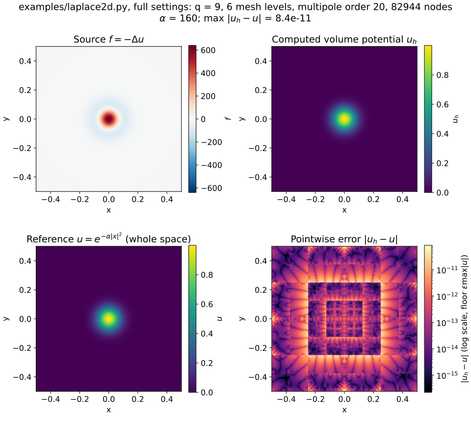
Computed by examples/laplace2d.py at full settings (quadrature order 9,
6 mesh levels, multipole order 20, 82944 quadrature nodes): the source
\(f = -\Delta u\), the computed potential \(u_h\), the whole-space reference
\(u = e^{-160 \lVert \boldsymbol{x} \rVert^2}\), and \(|u_h - u|\), whose maximum
over the nodes the example printed as Error = 8.410442587858608e-11.
Regenerate with
python doc/tools/render_gallery.py laplace2d --pyopencl-ctx portable:0 --full.#
Reproduce the figure above, then read the program behind it in six short steps: source, quadrature nodes, tree, near-field table, FMM, error.
Computed figures from the maintained examples, in two and three dimensions, each with the settings and the command that produced it.
The name is short for VOLUME poteNTIAL. For a kernel \(G\) and a source density \(f\) on a box-shaped domain \(\Omega\), Volumential evaluates
The far field is an ordinary particle FMM over the volume quadrature nodes;
the near field is read from precomputed, symmetry-reduced interaction tables.
That split — far field by particle approximation, near field direct — is
what the code calls the fpnd strategy, and it is the thing most of this
documentation is about.
Supported kernels are Laplace, Helmholtz and Yukawa (modified Helmholtz) in two and three dimensions, with potential and target-gradient outputs, on uniform and adaptively refined 2:1-balanced trees.
Install the stack, evaluate a first volume potential, and pick the OpenCL device you meant to use.
Run commands, smoke modes, cost classes, caches and device behavior for every maintained program and notebook; the gallery above is the visual map.
The volume-FMM workflow end to end: meshes and trees, near-field tables and their symmetry reduction, the Helmholtz split, derivatives, and what is validated.
Short accounts of the two mechanisms that are easiest to misread from the source alone: windowed singular channels with certified assembly, and ORBIT canonicalization.
What a measurement of this library has to record to be worth quoting: the resolved device, the revision, the parameters, first call versus warm.
One generated page per module, with a map from the pieces of the volume FMM to the module that owns them.
Contributing, the test tiers and their markers, CI and the review bots, and release and versioning.
Where to start#
Never run Volumential before: Installation, then A first volume potential.
Looking for a program close to your problem: Visual gallery, then Examples for run/cost/cache details.
Want to understand the machinery: The volume-FMM workflow.
Chasing a slow or wrong table: Near-field table build routing and Near-Field Symmetry Reduction.
Measuring, or quoting a measurement: Benchmarks and reproducibility.