Visual gallery#
If you are deciding whether Volumential fits a problem, start here rather than
with the API reference. The first four cards show the committed output of a
maintained example, rendered at the example’s full settings by
doc/tools/render_gallery.py, with the settings, the numbers the run printed,
and the command that regenerates the figure. The near/far card is a
schematic and says so; the Poisson 2-D card has no figure and says why. A
thumbnail is a crop: select it to open the full figure. The documentation
build runs none of these examples.
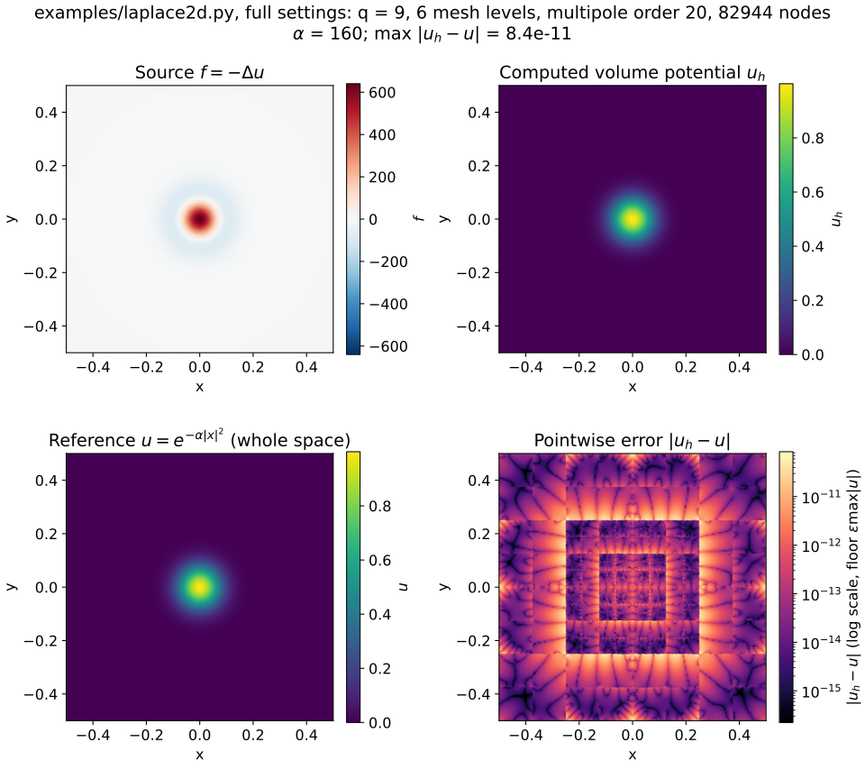
Start here. The source \(f = -\Delta u\), the computed potential \(u_h\), the whole-space Gaussian reference \(u = e^{-160 \lVert \boldsymbol{x} \rVert^2}\) and the pointwise error \(|u_h - u|\) on \([-1/2, 1/2]^2\).
examples/laplace2d.py, full settings: quadrature order 9, 6 mesh levels,
multipole order 20, 82944 quadrature nodes. The run printed
Error = 8.410442587858608e-11, the maximum of \(|u_h - u|\) over the nodes.
python doc/tools/render_gallery.py laplace2d \
    --pyopencl-ctx portable:0 --full
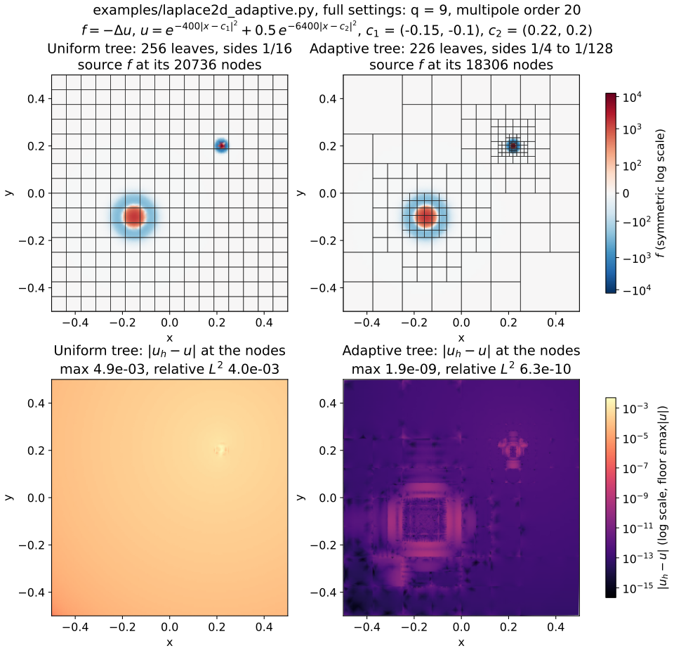
What an adaptive tree buys. The source \(f = -\Delta u\) for \(u = e^{-400 \lVert \boldsymbol{x} - \boldsymbol{c}_1 \rVert^2} + 0.5\, e^{-6400 \lVert \boldsymbol{x} - \boldsymbol{c}_2 \rVert^2}\), a broad Gaussian at \(\boldsymbol{c}_1 = (-0.15, -0.1)\) and a narrow one at \(\boldsymbol{c}_2 = (0.22, 0.2)\) in \([-1/2, 1/2]^2\), computed twice with the same quadrature order, near-field table and multipole order: on a uniform tree, and on an adaptive tree allowed at most as many leaves. The top row shows each tree over the source at its nodes, the bottom row \(|u_h - u|\) at those nodes. The reference \(u\) is the whole-space solution; both Gaussians are below \(e^{-40}\) outside the square, so the source the square leaves out is far below the errors shown.
The uniform leaves, 1/16 of the square across, are too coarse for the narrow Gaussian, and what they miss of it is felt across the whole square through the potential. The adaptive tree keeps leaves 1/8 and 1/4 across where the source is flat and goes down to 1/128 around the narrow Gaussian.
examples/laplace2d_adaptive.py, full settings: quadrature order 9,
multipole order 20. The run printed, for the uniform tree, 256 leaves and
20736 nodes, a maximum of \(|u_h - u|\) over the nodes of 4.880e-03 and a
relative \(L^2\) error of 3.960e-03; for the adaptive tree, after 16
refinement passes, 226 leaves and 18306 nodes, 1.949e-09 and 6.325e-10.
It then printed the same for finer uniform trees: 6.970e-06 and 1.589e-06
with 1024 leaves and 82944 nodes, 6.442e-09 and 9.729e-10 with 4096 leaves
and 331776 nodes. Only at \(64 \times 64\) leaves does the uniform tree come
close to the adaptive tree’s accuracy, and it still falls short of it.
python doc/tools/render_gallery.py laplace2d-adaptive \
    --pyopencl-ctx portable:0 --full
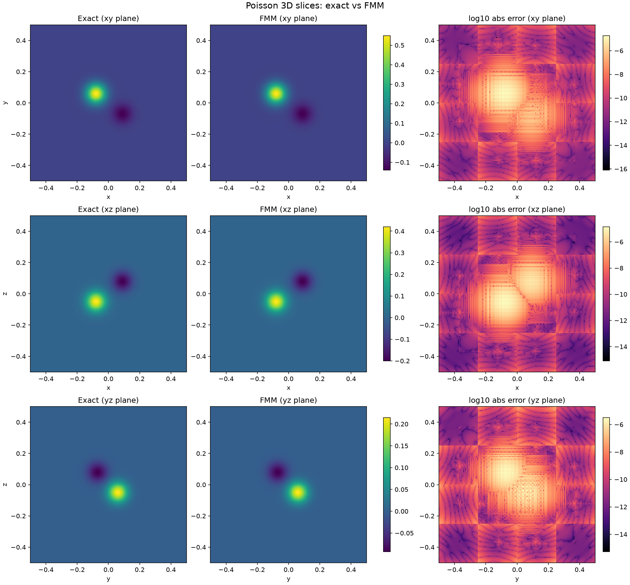
Two Gaussians of opposite sign, each \(e^{-240 r^2}\), on \([-1/2, 1/2]^3\), cut by the planes \(z = 0\), \(y = 0\) and \(x = 0\). The columns are the manufactured solution (titled “Exact”), the FMM potential interpolated to 180 × 180 points per plane, and \(\log_{10}\) of their difference. “Exact” is the whole-space solution of \(-\Delta u = f\), while the example integrates over the cube only; both Gaussians are below \(e^{-40}\) on the cube’s boundary, so the source left out is far below the errors shown. The error is largest around the two Gaussians and falls by several orders of magnitude away from them, in blocks that follow the boxes of the tree.
examples/poisson3d.py, full settings: quadrature order 7, 5 mesh levels
(16³ leaf cells), multipole order 16, near-field table quadrature orders 16
(regular) and 80 (radial). At the quadrature nodes the run printed a maximum
absolute error of 5.768837e-07 and a relative L2 error of 1.190132e-07.
The slices reach about \(10^{-5}\) because they add interpolation from the nodes
to the points between them.
python doc/tools/render_gallery.py poisson3d \
    --pyopencl-ctx portable:0 --full
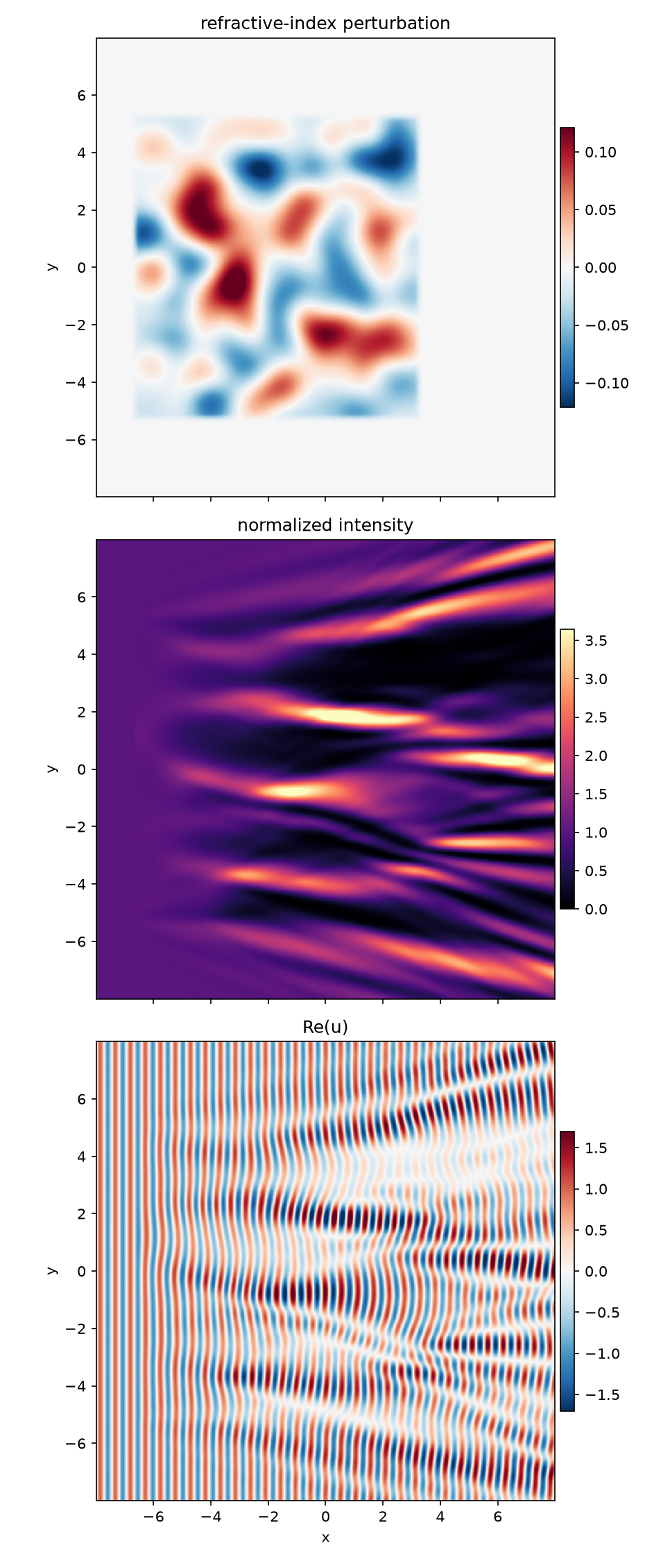
A plane wave with \(k = 12\), incident along \(+x\), through a smooth random medium, solved as a free-space Lippmann–Schwinger equation on \([-8, 8]^2\) with no artificial boundary or PML. The figure stacks the refractive-index perturbation \(n - 1\), the intensity \(|u|^2\) normalized by the mean incident intensity, and \(\operatorname{Re} u\); each color scale is clipped at the 99.5th percentile of the plotted magnitude. The thumbnail shows the intensity, where the wave breaks into branching filaments that keep spreading past the medium.
examples/branched_flow_helmholtz2d.py, default (full) configuration:
quadrature order 4, 9 levels, 1048576 points, the fmmlib far field, GMRES
to a tolerance of \(10^{-8}\) without a preconditioner. The medium is a sum of
2048 Gaussian bumps of width 0.55 (the example’s correlation_length
parameter; refractive-index RMS 0.05, seed 17) on \([-6.4, 3] \times [-5, 5]\),
faded out over a layer of width 0.5. The run printed 34 GMRES iterations and a
relative true residual of 9.567252072103188e-09. It needs pyfmmlib.
python doc/tools/render_gallery.py branched-flow \
    --pyopencl-ctx portable:0 --full
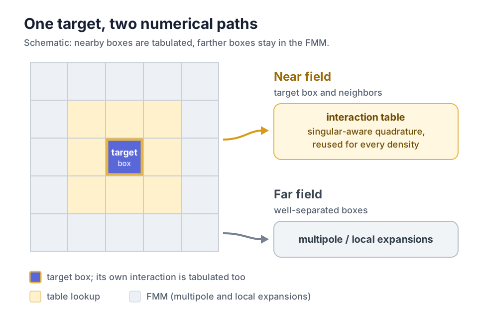
Schematic, not computed output. Why the singular neighborhood of a target box leaves the ordinary particle FMM path, what is tabulated, and what can be reused when the source density changes. Read it before the detailed implementation pages.
The diagram is drawn by hand and edited directly in
doc/source/gallery/near-far-anatomy.svg.
No figure. The notebook poisson2d_pytential_volumential.ipynb couples
Volumential to Pytential, enforces Dirichlet data with a harmonic boundary
correction, and compares uniform refinement with boundary-focused adaptive
refinement. Its figures exist only when the notebook runs: it is committed
without outputs, the documentation does not execute notebooks, and no
maintained script produces them, so there is no computed figure to show here.
Run the notebook to see them. For an adaptive tree and what it buys over a
uniform one, see the adaptive refinement card above, a smaller problem: a
source in the square, with no boundary to fit.
Which example should I copy?#
New to the library: A first volume potential.
A source with local features, on an adaptive tree:
laplace2d_adaptive.py.A 3-D manufactured solve with spatial error diagnostics:
poisson3d.py.Volume and boundary integral machinery together, on a curved domain: the 2-D Poisson notebook.
Helmholtz with the Laplace-table smooth correction:
helmholtz2d.pyorhelmholtz3d.py, which are convergence studies in the quadrature order.A large scattering application:
branched_flow_helmholtz2d.py.
Use the convergence studies for numerical behavior, and read Benchmarks and reproducibility before quoting a timing.
Regenerate the figures#
The documentation build deliberately runs no scientific workload; it only
shows the files committed under doc/source/gallery/. All of the computed
figures above come from one command, run in the Volumential environment with
matplotlib (and pyfmmlib for branched flow) installed:
python doc/tools/render_gallery.py all --full --pyopencl-ctx portable:0
The command on each card regenerates that figure alone. Without --full the
renderer uses the examples’ smoke settings, which run in seconds and show that
the figure path works but do not resolve the problems, so their figures are
not results. doc/source/gallery/manifest.json records the revision, command,
environment, device type and package versions behind each computed figure,
and Gallery assets describes the renderer and the rules
for changing a figure.
Need the operational details?#
The main Examples page remains the source of truth for cache filenames, device-selection behavior, smoke modes and the cost class of every example.