A first volume potential#

This page runs the maintained example examples/laplace2d.py, shows what it computes, and then takes the program apart in six steps.

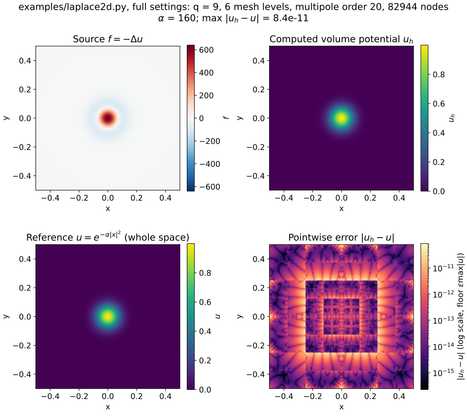
Four panels over the square: the source, the computed potential, the Gaussian reference, which looks identical, and the pointwise error on a logarithmic scale, at most about 8e-11. — The run this page builds, computed by `examples/laplace2d.py` at full settings: quadrature order 9, 6 mesh levels, multipole order 20, 82944 quadrature nodes, \(\alpha = 160\). Top: the source \(f\) and the computed potential \(u_h\). Bottom: the reference \(u\), on the same color scale as \(u_h\), and \(|u_h - u|\) on a logarithmic scale whose floor is machine epsilon times \(\max |u|\). Regenerate with `python doc/tools/render_gallery.py laplace2d --pyopencl-ctx portable:0 --full`.#

The example evaluates the Laplace volume potential of a source \(f\) over the square \([-1/2, 1/2]^2\),

\[ v(\boldsymbol{x}) = \int_{[-1/2,\,1/2]^2} \frac{-1}{2\pi} \log \lVert \boldsymbol{x} - \boldsymbol{y} \rVert \, f(\boldsymbol{y}) \, \mathrm{d}\boldsymbol{y}, \]

where \(f = -\Delta u\) for the Gaussian \(u(\boldsymbol{x}) = e^{-\alpha \lVert \boldsymbol{x} \rVert^2}\). Because \(-\frac{1}{2\pi} \log \lVert \boldsymbol{x} \rVert\) is the fundamental solution of \(-\Delta\), \(u\) is what the integral gives over the whole plane. Over the square, \(v\) differs from \(u\) only by the source the square leaves out, and outside the square the Gaussian factor is below \(e^{-40}\), so that difference is at rounding level. \(u\) is therefore a reference for \(v\) at every quadrature node, and \(|u_h - u|\) measures the error of the computed potential \(u_h\). That is what makes this a useful first run: the answer can be checked, not only looked at.

Run it#

Set PYOPENCL_CTX before running it. Otherwise cl.create_some_context() stops and asks which device to use at a terminal, and picks one in an implementation-defined manner anywhere else:

export PYOPENCL_CTX=portable:0
uv run python examples/laplace2d.py

The first run builds the near-field table and caches it in nft_laplace2d.sqlite in the working directory; later runs load it. After the FMM the example prints the maximum of \(|u_h - u|\) over the quadrature nodes. The run behind the figure printed

Error = 8.410442587858608e-11

and a different device or library version may change the trailing digits.

To write the two figures on this page from your own run, point VOLUMENTIAL_GALLERY_OUTPUT_DIR at a directory. The figures need matplotlib; the setting does not change the computation, and the example writes the figures from the data it has already computed:

VOLUMENTIAL_GALLERY_OUTPUT_DIR=build/gallery/laplace2d \
uv run --with matplotlib python examples/laplace2d.py

VOLUMENTIAL_EXAMPLE_SMOKE=1 switches to quadrature order 3, two mesh levels and multipole order 8, with a separate cache file. That is what CI runs. It checks that the stack works end to end, but it does not resolve the Gaussian: its error is of order one, so treat it as a setup check and not as an accuracy result.

VOLUMENTIAL_EXAMPLE_SMOKE=1 uv run python examples/laplace2d.py

The program in six steps#

The complete program is at the end of this section. The six steps below are the parts that matter; the rest constructs objects and moves arrays between host and device.

1. Describe the source#

x, y, exp = pmbl.var("x"), pmbl.var("y"), pmbl.var("exp")
norm2 = x**2 + y**2
source_expr = -(4 * alpha**2 * norm2 - 4 * alpha) * exp(-alpha * norm2)

This is the top-left panel of the figure: \(f = -\Delta u\) as a symbolic expression, evaluated at the quadrature nodes in the next step.

2. Put quadrature nodes in boxes#

mesh = mg.MeshGen2D(q_order, n_levels, -0.5, 0.5, queue=queue)
nodes = np.ascontiguousarray(mesh.get_q_points().T)
source_vals = cl.array.to_device(
    queue, Eval(dim, source_expr, [x, y])(queue, nodes))

MeshGen2D splits the square into \(2^{\,n_\mathrm{levels} - 1}\) intervals per axis, 32 × 32 leaf boxes here, and puts a tensor-product Gauss–Legendre rule of order q_order in each: 81 nodes per box, 82944 in all.

3. Build the tree#

_, q_weights, tree, trav = mg.build_geometry_info(
    ctx, queue, dim, q_order, mesh, bbox=np.array([[-0.5, 0.5]] * dim))

build_geometry_info builds the FMM tree from the mesh’s own boxes, so that every leaf is a mesh cell holding its 81 nodes, which is the geometry the near-field table assumes. A tree built from the nodes alone would take their extent, not the square, as its root box, and its leaves would not coincide with the mesh cells. The call then builds the traversal, which records for every box the boxes near it and the ones well separated from it, and returns the quadrature weights on the device.

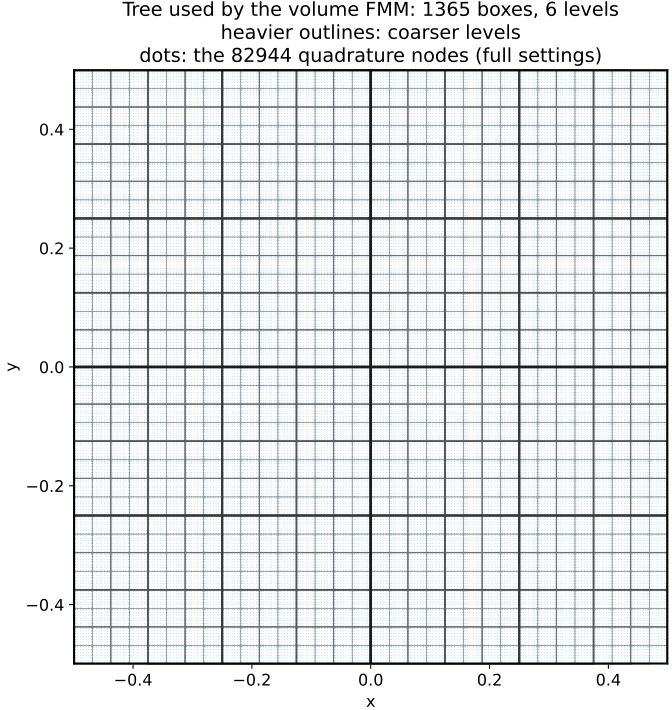
The square from -0.5 to 0.5 divided uniformly into a 32 by 32 grid of leaf boxes, with the outlines of the coarser boxes drawn over it and the quadrature nodes as faint dots. — The tree of the run at the top: 1365 boxes on 6 levels, coarser levels drawn with heavier outlines, and the 82944 quadrature nodes as dots. The tree is uniform because the example’s mesh is uniform. Computed by `examples/laplace2d.py` at full settings in the same run as the first figure, and regenerated by the same command.#

4. Get the near-field table#

tm = NearFieldInteractionTableManager(
    "nft_laplace2d.sqlite", root_extent=2, queue=queue)
build_config = DuffyBuildConfig(
    radial_rule="tanh-sinh-fast",
    regular_quad_order=50, radial_quad_order=100)
nftable, _ = tm.get_table(
    dim, "Laplace", q_order, queue=queue, build_config=build_config)

On a cache miss this builds the table by Duffy-transformed quadrature and writes it to the SQLite file; later runs load it. build_config is the quadrature the example uses for that build. A cached table built with a different configuration is rebuilt rather than reused.

5. Give the FMM a different near-field rule#

The wrangler uses ordinary sumpy multipole and local expansions for the far field, but substitutes the table for the point-to-point near-field stage. That substitution is the part specific to Volumential; the complete program below shows how the wrangler is constructed.

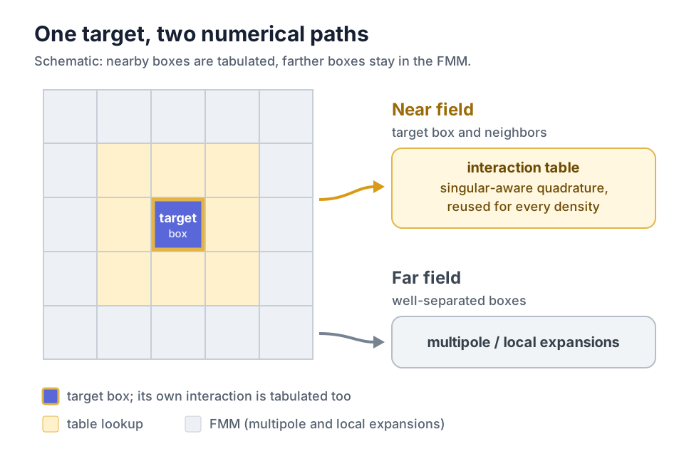
Schematic. A five by five block of boxes. The target box and its eight neighbors are table lookups, the target box's own interaction included; the outer ring is handled by the FMM with multipole and local expansions. — Schematic, not computed output. For one target box, the box itself and its eight neighbors are served by the near-field interaction table, and the well-separated boxes by the FMM. Anatomy of a near-field interaction explains the picture.#

6. Drive the FMM and check the answer#

(pot,) = drive_volume_fmm(
    trav, wrangler, source_vals * q_weights, source_vals)

reference = np.exp(-alpha * (nodes[0] ** 2 + nodes[1] ** 2))
print("max error =", np.max(np.abs(pot.get() - reference)))

The two source arrays differ on purpose. source_vals * q_weights is what the far field sums as particle strengths; source_vals is the bare density the near-field table is contracted against. Passing the same array for both is a quiet error.

The bottom-right panel of the figure at the top is this difference at every node. It is at most \(8.4 \times 10^{-11}\) in that run, and it is not uniform: it jumps across box edges, and its nested squares line up with the boxes of the tree in step 3.

Complete program

from functools import partial

import numpy as np
import pymbolic as pmbl
import pyopencl as cl
import pyopencl.array  # noqa: F401
from sumpy.expansion import DefaultExpansionFactory
from sumpy.kernel import LaplaceKernel

import volumential.meshgen as mg
from volumential.expansion_wrangler_fpnd import (
    FPNDExpansionWrangler, FPNDTreeIndependentDataForWrangler)
from volumential.nearfield_potential_table import DuffyBuildConfig
from volumential.table_manager import NearFieldInteractionTableManager
from volumential.tools import ScalarFieldExpressionEvaluation as Eval
from volumential.volume_fmm import drive_volume_fmm

dim, q_order, n_levels, m_order, alpha = 2, 9, 6, 20, 160
ctx = cl.create_some_context()
queue = cl.CommandQueue(ctx)

# 1. The source density, as a symbolic expression evaluated on device.
x, y, exp = pmbl.var("x"), pmbl.var("y"), pmbl.var("exp")
norm2 = x**2 + y**2
source_expr = -(4 * alpha**2 * norm2 - 4 * alpha) * exp(-alpha * norm2)

# 2. A box mesh over [-1/2, 1/2]^2 and its volume quadrature nodes.
mesh = mg.MeshGen2D(q_order, n_levels, -0.5, 0.5, queue=queue)
nodes = np.ascontiguousarray(mesh.get_q_points().T)
source_vals = cl.array.to_device(
    queue, Eval(dim, source_expr, [x, y])(queue, nodes))

# 3. The FMM tree, built from the mesh's boxes, and its traversal.
_, q_weights, tree, trav = mg.build_geometry_info(
    ctx, queue, dim, q_order, mesh, bbox=np.array([[-0.5, 0.5]] * dim))

# 4. The near-field interaction table, built once and cached in SQLite.
tm = NearFieldInteractionTableManager(
    "nft_laplace2d.sqlite", root_extent=2, queue=queue)
build_config = DuffyBuildConfig(
    radial_rule="tanh-sinh-fast",
    regular_quad_order=50, radial_quad_order=100)
nftable, _ = tm.get_table(
    dim, "Laplace", q_order, queue=queue, build_config=build_config)

# 5. The wrangler: sumpy expansions for the far field, the table for the near.
knl = LaplaceKernel(dim)
factory = DefaultExpansionFactory()
tree_indep = FPNDTreeIndependentDataForWrangler(
    ctx,
    partial(factory.get_multipole_expansion_class(knl), knl),
    partial(factory.get_local_expansion_class(knl), knl),
    [knl],
    exclude_self=True)
wrangler = FPNDExpansionWrangler(
    tree_indep=tree_indep, queue=queue, traversal=trav,
    near_field_table=nftable, dtype=np.float64,
    fmm_level_to_order=lambda *args: m_order, quad_order=q_order,
    self_extra_kwargs={
        "target_to_source": np.arange(tree.ntargets, dtype=np.int32)})

# 6. Evaluate, and compare with the whole-space Gaussian.
(pot,) = drive_volume_fmm(
    trav, wrangler, source_vals * q_weights, source_vals)

reference = np.exp(-alpha * (nodes[0] ** 2 + nodes[1] ** 2))
print("max error =", np.max(np.abs(pot.get() - reference)))

This program computes the same potential as examples/laplace2d.py, with the same settings, tree and table configuration, and shares its cache file. The maintained example adds the figure output, and carries a multilevel-table variant and a direct point-to-point check, both switched off.

What just happened#

Step 2 turns the integral into weighted point sources, source_vals * q_weights, which the far field sums like particles. Steps 4 and 5 are what make the result a volume potential rather than a particle sum: for the target box and its neighbors, where point quadrature converges too slowly and erratically to be usable, FPNDExpansionWrangler takes the interaction from the table instead. Anatomy of a near-field interaction explains why.

Step 4 is where the cost is. The first run builds the near-field table by Duffy-transformed quadrature and writes it to nft_laplace2d.sqlite; later runs load it in milliseconds. The table depends on the kernel, the dimension, q_order and the scale of the source box — the manager’s root_extent and the request’s source_box_level, from which source_box_extent is derived — but not on the source density, the tree’s topology or the target points. So the cache file is worth keeping and reusing across runs of this example, and is not reusable at a different root extent. See Near-field table build routing for how a build is routed and how to tell a cached table’s provenance, and Near-Field Symmetry Reduction for why the stored table is much smaller than the number of interactions it serves.

Next#

Computed figures from the other maintained examples, and the command behind each: Visual gallery.
The same kind of run on an adaptive tree, which puts its leaves where the source needs them, next to the uniform tree it replaces: examples/laplace2d_adaptive.py, and its card in Visual gallery.
The near/far split without the API: Anatomy of a near-field interaction.
Other maintained examples: examples/laplace3d.py, examples/helmholtz2d.py, examples/helmholtz3d.py, examples/poisson3d.py and examples/branched_flow_helmholtz2d.py. All of them read PYOPENCL_CTX. Without it, the three Helmholtz scripts pick their own device, preferring an fp64 GPU — see Device selection.
Choosing the device the run lands on: Device selection.
The whole pipeline, stage by stage: The volume-FMM workflow.